Best Practices Guide

Introduction

This chapter covers a number of best practices for the PhysX SDK to assist in diagnosing and fixing frequently encountered issues.

Debugging

The PhysX SDK contains a few debugging helpers. They can be used to make sure the scenes are properly set up.

Use checked builds and the error stream

The PhysX SDK has different build configurations: Debug, Checked, Release, Profile. To make sure that the scene is properly set up without warnings or errors, use either the Debug or Checked builds, and monitor the error callback. Please refer to the Error Reporting chapter for details. Note that some checks can be expensive and thus they are not performed in Release or Profile builds. If the SDK silently fails or even crashes in a Release build, please switch to Debug or Checked builds to ensure this is not caused by an uncaught error.

Visualizing physics data

Use the PhysX Visual Debugger (PVD) to see what PhysX is seeing and make sure the physics data is what you expect it to be. Please refer to the PhysX Visual Debugger (PVD) chapter for details. Note that this is only available in Debug, Checked and Profile builds.

Visualizing physics data (2)

An alternative to PVD is the built-in debug visualization system. Please refer to the Debug Visualization chapter for details. This option is available with all build configurations.

Limiting coordinates

Bugs in applications, or issues in content creation, can sometimes result in object placement at unexpected coordinates. We recommend the use of PxSceneDesc::sanityBounds, to generate reports when objects are inserted at positions beyond what your application expects, or when application code moves them to such unexpected positions. Note that these bounds only apply to application updates of actor coordinates, not updates by the simulation engine.

Performance Issues

The PhysX SDK has been optimized a lot in the past dot releases. However, there still exist various performance pitfalls that the user should be aware of.

Use profile builds to identify performance bottlenecks

The PhysX SDK has different build configurations: Debug, Checked, Release, Profile. To identify performance bottlenecks, please use Profile builds and PVD. Use the PxPvdInstrumentationFlag::ePROFILE only, since enabling the other connection flags might negatively affect performance. Please refer to the PhysX Visual Debugger (PVD) chapter for details.

Use release builds for final performance tests

The PhysX SDK has different build configurations: Debug, Checked, Release, Profile. The Release builds are the most optimal. If you encounter a performance issue while using other builds, please switch to Release builds and check if the problem is still there.

Disable debug visualization in final/release builds

Debug visualization is great for debugging but it can have a significant performance impact. Make sure it is disabled in your final/release builds. Please refer to the Debug Visualization chapter for details.

Debug visualization is very slow

Debug visualization can be very slow, because both the code gathering the debug data and the code rendering it is usually not optimal. Use a culling box to limit the amount of data the SDK gathers and sends to the renderer. Please refer to the Debug Visualization chapter for details.

Consider using tight bounds for convex meshes

By default PhysX computes approximate (loose) bounds around convex objects. Using PxConvexMeshGeometryFlag::eTIGHT_BOUNDS enables smaller/tighter bounds, which are more expensive to compute but can result in improved simulation performance when a lot of convex objects are interacting with each other. Please refer to the Geometry chapter for details.

Use scratch buffers

The PxScene::simulate function accepts optional scratch buffers that can be used to reduce temporary allocations and improve simulation performance. Please refer to the Simulation chapter for details.

Use the proper mid-phase algorithm

PxCookingParams::midphaseDesc can be used to select the desired mid-phase structure. It is a good idea to try the different options and see which one works best for you. Generally speaking the new PxMeshMidPhase::eBVH34 introduced in PhysX 3.4 has better performance for scene queries against large triangle meshes. Please refer to the Geometry chapter for details.

Use the proper narrow-phase algorithm

PxSceneFlag::eENABLE_PCM enables an incremental "persistent contact manifold" algorithm, which is often faster than the previous implementation. PCM should be the default algorithm since PhysX 3.4, but you can also try to enable it in previous versions like 3.3.

Use the proper broad-phase algorithm

PhysX also supports two different broad-phase implementations, selected with PxSceneDesc::broadPhaseType. The different implementations have various performance characteristics, and it is a good idea to experiment with both and find which one works best for you. Please refer to the Rigid Body Collision chapter for details about the different broad-phases.

Use the scene-query and simulation flags

If a shape is only used for scene-queries (raycasts, etc), disable its simulation flag. If a shape is only used for simulation (e.g. it will never be raycasted against), disable its scene-query flag. This is good for both memory usage and performance. Please refer to the Rigid Body Collision chapter for details.

Tweak the dynamic tree rebuild rate

If the PxScene::fetchResults call takes a significant amount of time in scenes containing a lot of dynamic objects, try to increase the PxSceneDesc::dynamicTreeRebuildRateHint parameter. Please refer to the Scene Queries chapter for details.

Use the insertion callback when cooking at runtime

Use PxPhysicsInsertionCallback for objects that are cooked at runtime. This is faster than first writing the data to a file or a memory buffer, and then passing the data to PhysX.

Kill kinematic pairs early

If you do not need them, use PxPairFilteringMode::eKILL to disable kinematic pairs earlier in the pipeline.

The "Well of Despair"

One common use-case for a physics engine is to simulate fixed-size time-steps independent of the frame rate that the application is rendered at. If the application is capable of being rendered at a higher frequency than the simulation frequency, the user has the option to render the same simulation state, interpolate frames etc. However, sometimes it is not possible to render the scene at a frequency higher-or-equal to the simulation frequency. At this point, the options are to either run the physics simulation with a larger time-step or to simulate multiple, smaller sub-steps. The latter is generally a preferable solution because changing the size of time-steps in a physics simulation can significantly change perceived behavior. However, when using a sub-stepping approach, one must always be aware of the potential that this has to damage performance.

As an example, let's imagine a game that is running using v-sync at 60FPS. This game is simulating a large number of physics bodies and, as a result, the physics is relatively expensive. In order to meet the 60FPS requirement, the entire frame must be completed within ~16ms. As already mentioned, the physics is reasonably expensive and, in this scenario, takes 9ms to simulate 1/60th of a second. If the game was to suddenly spike, e.g. as a result of some OS activity, saving a check-point or loading a new section of the level, we may miss the deadline for 60FPS. If this happens, we must run additional sub-steps in the physics to catch up the missed time in the next frame. Assuming that the previous frame took 50ms instead of 16ms, we must now simulate 3 sub-steps to be able to simulate all the elapsed time. However, each sub-step takes ~9ms, which means that we will take ~27ms to simulate 50ms. As a result, this frame also misses our 16ms deadline for 60FPS, meaning that the frame including v-sync took 33ms (i.e. 30Hz). We must now simulate 2 sub-steps in the next frame, which takes ~18ms and also misses our 16ms deadline. As a result, we never manage to recover back to 60FPS. In this scenario, our decision to sub-step as a result of a spike has resulted in our application being stuck in a performance trough indefinitely. The application is capable of simulating and rendering at 60FPS but becomes stuck in the so-called "physics well of despair" as a result of substepping.

Problems like this can be alleviated in several ways:

• Decouple the physics simulation from the game's update/render loop. In this case, the physics simulation becomes a scheduled event that occurs at a fixed frequency. This can make player interaction in the scene more difficult and may introduce latency so must be well-thought through. However, using multiple scenes (one synchronous for "important" objects, one asynchronous for "unimportant" objects) can help.
• Permit the game to "drop" time when faced with a short-term spike. This may introduce visible motion artifacts if spikes occur frequently.
• Introduce slight variations in time-step (e.g. instead of simulating at 1/60th, consider simulating a range between 1/50th and 1/60th). This can introduce non-determinism into the simulation so should be used with caution. If this is done, additional time that must be simulated can potentially be amortized over several frames by simulating slightly larger time-steps.
• Consider simplifying the physics scene, e.g. reducing object count, shape complexity, adjusting iteration counts etc. Provided physics simulation is a small portion of the total frame time, the application should find it easier to recover from spikes.

Pruner Performance for Streamed Environments

PhysX provides multiple types of pruners, each of which aimed at specific applications. These are:

• Static AABB tree
• Dynamic AABB tree

By default, the static AABB tree is used for the static objects in the environment and the dynamics AABB tree is used for the dynamic objects in the environment. In general, this approach works well but it must be noted that creating the static AABB tree can be very expensive. As a result, adding, removing or moving any static objects in the environment will result in the static AABB tree being fully recomputed, which can introduce significant performance cost. As a result, we recommend the use of dynamics AABB trees for both static and dynamic pruners in games which stream in the static environment. Additionaly scene query performance against newly added objects can be improved by using PxPruningStructure, which can precompute the AABB structure of inserted objects in offline.

Performance Implications for Multi-Threading

The PhysX engine is designed from the ground-up to take advantage of multi-core architectures to accelerate physics simulation. However, this does not mean that more threads are always better. When simulating extremely simple scenes, introducing additional worker threads can detrimentally affect performance. This is because, at its core, PhysX operates around a task queue. When a frame's simulation is started, PhysX dispatches a chain of tasks that encapsulate that frame of physics simulation. At various stages of the physics pipeline, work can be performed in parallel on multiple worker threads. However, if there is insufficient work, there will be little or no parallel execution. In this case, the use of additional worker threads may detrimentally affect performance because the various phases of the pipeline may be run by different worker threads, which may incur some additional overhead depending on the CPU architecture compared to running on just a single worker thread. As a result, developers should measure the performance of the engine with their expected physics loads with different numbers of threads to maximize their performance and make sure that they are making the most of the available processing resources for their game.

Memory allocation

Minimizing dynamic allocation is an important aspect of performance tuning, and PhysX provides several mechanisms to control memory usage.

Reduce allocation used for tracking objects by presizing the capacities of scene data structures, using either PxSceneDesc::limits before creating the scene or the function PxScene::setLimits(). When resizing, the new capacities will be at least as large as required to deal with the objects currently in the scene. These values are only for preallocation and do not represent hard limits, so if you add more objects to the scene than the capacity limits you have set, PhysX will allocate more space.

Much of the memory PhysX uses for simulation is held in a pool of blocks, each 16K in size. You can control the current and maximum size of the pool with the nbContactDataBlocks and maxNbContactDataBlocks members of PxSceneDesc. PhysX will never allocate more than the maximum number of blocks specified, and if there is insufficient memory it will instead simply drop contacts or joint constraints. You can find out how many blocks are currently in use with the getNbContactBlocksUsed() method, and find out the maximum number that have ever been used with the getMaxNbContactDataBlocksUsed() method.

Use PxScene::flushSimulation() to reclaim unused blocks, and to shrink the size of scene data structures to the size presently required.

To reduce temporary allocation performed during simulation, provide physx with a memory block in the simulate() call. The block may be reused by the application after the fetchResults() call which marks the end of simulation. The size of the block must be a multiple of 16K, and it must be 16-byte aligned.

Character Controller Systems using Scene Queries and Penetration Depth Computation

Implementing a Character Controller (CCT) is a common use case for the PhysX Scene Query (SQ) system. A popular approach is to use sweeps to implement movement logic, and to improve robustness by using Geometry Queries (GQ) to compute and resolve any penetrations that occur due to object movement that does not account for the presence of the controller, or due to numerical precision issues.

Basic Algorithm:

1. Call a SQ-Sweep from the current position of the CCT shape to its goal position.
2. If no initial overlap is detected, move the CCT shape to the position of the first hit, and adjust the trajectory of the CCT by removing the motion relative to the contact normal of the hit.
3. Repeat Steps 1 and 2 until the goal is reached, or until an SQ-Sweep in Step 1 detects an initial overlap.
4. If an SQ-Sweep in Step 1 detects an initial overlap, use the GQ Penetration Depth computation function to generate a direction for depenetration. Move the CCT shape out of penetration and begin again with Step 1.

Limitations and Problems

Step 4 of the algorithm above can sometimes run into trouble due to implementation differences in SQ-Sweep, SQ-Overlap and and GQ-Penetration Depth queries. Under certain initial conditions it is possible that the SQ system will determine that a pair of objects is initially overlapping while the GQ -Penetration Depth computation will report them as disjoint (or vice-versa). Penetration depth calculations involving convex hulls operate by shrinking the convex hull and performing distance calculations between a shape and the shrunken convex hull. To understand the conditions under which this occurs and how to resolve the artefacts, please refer to the diagrams and discussion below. Each diagram represents the initial conditions of two shapes, a Character Controller shape (red boxes), a convex obstacle (black boxes), at the time that Step 1 of the algorithm above is executed. In the diagrams, the outermost rectangular black box is the convex hull as seen by the SQ algorithms; the inner black box with a dashed line represents the shrunken convex shape and the black box with rounded corners is the shrunken convex shape inflated by the amount by which we shrunk. These three black boxes are used by the GQ-Penetration Depth computation. Although the example refers to convex hull obstacles, the issue is not exclusive to the convex hull shapes; the problem is similar for other shape types as well.

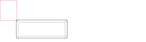
Diagram 1: CCT Shape Barely Touches an Obstacle

In Diagram 1, the red box of the CCT is barely touching the outermost black box of the convex obstacle. In this situation the SQ-Sweep will report an initial overlap but the GQ-Penetration Depth function will report no hit, because the red box is not touching the black box with rounded corners.

To resolve this, inflate the CCT shape for the GQ-Penetration Depth calculation to ensure that it detects an overlap and returns a valid normal. Note that after inflating the CCT shape, the GQ-Penetration Depth function will report that the shapes are penetrated more deeply than they actually are, so take this additional penetration into account when depenetrating in Step 4. This may result in some clipping around the corners and edges of convex objects but the CCT's motion should be acceptable. As the corners/edges become more acute, the amount of clipping will increase.

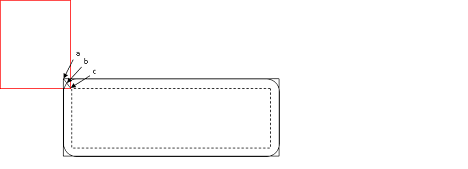
Diagram 2: CCT Overlaps an Obstacle Slightly

Diagram 2 shows a case where the CCT initially overlaps the outer black box seen by the SQ system, but does not overlap the shrunken shape seen by the GQ-Penetration Depth calculator. The GQ-Penetration Depth system will return the penetration from point c to point b but not from point c to point a. Therefore the CCT may clip through the corner of the convex hull after depenetration. This can be corrected in Step 4.

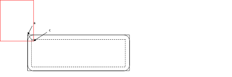
Diagram 3: CCT Overlaps an Obstacle Significantly

As can been seen from Diagram 3, if the CCT penetrates sufficiently that it overlaps with the shrunken shape seen by GQ, the GQ-Penetration Depth calculator will return the penetration from point c to point a. In this case, the GQ-Penetration Depth value can be used without modification in Step 4. However, as this condition would be difficult to categorize without additional computational cost, it is best to inflate the shape as recommended in Step 4 and then subtract this inflation from the returned penetration depth.

Unified MTD Sweep

A recent addition to the scene query sweeps is the flag PxHitFlag::eMTD. This can be used in conjunction with default sweeps to generate the MTD (Minimum Translation Direction) when an initial overlap is detected by a sweep. This flag is guaranteed to generate an appropriate normal under all circumstances, including cases where the sweep may detect an initial overlap but calling a stand-alone MTD function may report no hits. It still may suffer from accuracy issues with penetration depths but, in the cases outlined above around corners/edges, it will report a distance of 0 and the correct contact normal. This can be used to remove components of the sweep moving into the normal direction and then re-sweeping when attempting to implement a CCT. This also generates compound MTDs for meshes/heightfields, which means that it reports an MTD that de-penetrates the shape from the entire mesh rather than just an individual triangle, if such an MTD exists.

Quantizing HeightField Samples

Heightfield samples are encoded using signed 16-bit integers for the y-height that are then converted to a float and multiplied by PxHeightFieldGeometry::heightScale to obtain local space scaled coordinates. Shape transform is then applied on top to obtain world space location. The transformation is performed as follows (in pseudo-code):

localScaledVertex = PxVec3(row * desc.rowScale, PxF32(heightSample) * heightScale,
    col * desc.columnScale)
worldVertex = shapeTransform( localScaledVertex )

The following code snippet shows one possible way to build quantized unscaled local space heightfield coordinates from world space grid heights stored in terrainData.verts:

const PxU32 ts = ...; // user heightfield dimensions (ts = terrain samples)
// create the actor for heightfield
PxRigidStatic* actor = physics.createRigidStatic(PxTransform(PxIdentity));

// iterate over source data points and find minimum and maximum heights
PxReal minHeight = PX_MAX_F32;
PxReal maxHeight = -PX_MAX_F32;
for(PxU32 s=0; s < ts * ts; s++)
{
    minHeight = PxMin(minHeight, terrainData.verts[s].y);
    maxHeight = PxMax(maxHeight, terrainData.verts[s].y);
}

// compute maximum height difference
PxReal deltaHeight = maxHeight - minHeight;

// maximum positive value that can be represented with signed 16 bit integer
PxReal quantization = (PxReal)0x7fff;

// compute heightScale such that the forward transform will generate the closest point
// to the source
// clamp to at least PX_MIN_HEIGHTFIELD_Y_SCALE to respect the PhysX API specs
PxReal heightScale = PxMax(deltaHeight / quantization, PX_MIN_HEIGHTFIELD_Y_SCALE);

PxU32* hfSamples = new PxU32[ts * ts];

PxU32 index = 0;
for(PxU32 col=0; col < ts; col++)
{
    for(PxU32 row=0; row < ts; row++)
    {
        PxI16 height;
        height = PxI16(quantization * ((terrainData.verts[(col*ts) + row].y - minHeight) /
            deltaHeight));

        PxHeightFieldSample& smp = (PxHeightFieldSample&)(hfSamples[(row*ts) + col]);
        smp.height = height;
        smp.materialIndex0 = userValue0;
        smp.materialIndex1 = userValue1;
        if (userFlipEdge)
            smp.setTessFlag();
    }
}

// Build PxHeightFieldDesc from samples
PxHeightFieldDesc terrainDesc;
terrainDesc.format          = PxHeightFieldFormat::eS16_TM;
terrainDesc.nbColumns       = ts;
terrainDesc.nbRows          = ts;
terrainDesc.samples.data    = hfSamples;
terrainDesc.samples.stride  = sizeof(PxU32); // 2x 8-bit material indices + 16-bit height
terrainDesc.thickness       = -10.0f; // user-specified heightfield thickness
terrainDesc.flags           = PxHeightFieldFlags();

PxHeightFieldGeometry hfGeom;
hfGeom.columnScale = terrainWidth / (ts-1); // compute column and row scale from input terrain
                                            // height grid
hfGeom.rowScale    = terrainWidth / (ts-1);
hfGeom.heightScale = deltaHeight!=0.0f ? heightScale : 1.0f;
hfGeom.heightField = cooking.createHeightField(terrainDesc, physics.getPhysicsInsertionCallback());

delete [] hfSamples;

PxTransform localPose;
localPose.p = PxVec3(-(terrainWidth * 0.5f),    // make it so that the center of the
    minHeight, -(terrainWidth * 0.5f));         // heightfield is at world (0,minHeight,0)
localPose.q = PxQuat(PxIdentity);
PxShape* shape = PxRigidActorExt::createExclusiveShape(*actor, hfGeom, material, nbMaterials);
shape->setLocalPose(localPose);

Reducing memory usage

The following strategies can be used to reduce PhysX's memory usage.

Consider using tight bounds for convex meshes

See the above chapter about Performance Issues for details. Using tight bounds for convex meshes is mainly useful for performance, but it can also reduce the amount of pairs coming out of the broad-phase, which decreases the amount of memory needed to manage these pairs.

Use scratch buffers

See the above chapter about Performance Issues for details. Scratch buffers can be shared between multiple sub-systems (e.g. physics and rendering), which can globally improve memory usage. PhysX will not use less memory per-se, but it will allocate less of it.

Flush simulation buffers

Call the PxScene::flushSimulation function to free internal buffers used for temporary computations. But be aware that these buffers are usually allocated once and reused in subsequent frames, so releasing the memory might trigger new re-allocations during the next simulate call, which can decrease performance. Please refer to the Simulation memory chapter for details.

Use preallocation

Use PxSceneDesc::limits to preallocate various internal arrays. Preallocating the exact necessary size for internal buffers may use less memory overall than the usual array resizing strategy of dynamic arrays. Please refer to the Simulation memory chapter for details.

Tweak cooking parameters

Some cooking parameters have a direct impact on memory usage. In particular, PxMeshPreprocessingFlag::eDISABLE_ACTIVE_EDGES_PRECOMPUTE, PxCookingParams::suppressTriangleMeshRemapTable, PxBVH33MidphaseDesc::meshCookingHint, PxBVH33MidphaseDesc::meshSizePerformanceTradeOff, PxBVH34MidphaseDesc::numTrisPerLeaf, PxCookingParams::midphaseDesc, PxCookingParams::gaussMapLimit and PxCookingParams::buildTriangleAdjacencies can be modified to choose between runtime performance, cooking performance or memory usage.

Share shape and mesh data

Share the same PxConvexMesh and PxTriangleMesh objects between multiple shape instances if possible. Use shared shapes if possible. Please refer to the Rigid Body Collision chapter for details about shape sharing.

Use the scene-query and simulation flags

If a shape is only used for scene-queries (raycasts, etc), disable its simulation flag. If a shape is only used for simulation (e.g. it will never be raycasted against), disable its scene-query flag. This is good for both memory usage and performance. Please refer to the Rigid Body Collision chapter for details.

Kill kinematic pairs early

If you do not need them, use PxPairFilteringMode::eKILL to disable kinematic pairs earlier in the pipeline.

Behavior issues

Objects do not spin realistically

For historical reasons the default maximum angular velocity is set to a low value (7.0). This can artificially prevent the objects from spinning quickly, which may look unrealistic and wrong in some cases. Please use PxRigidDynamic::setMaxAngularVelocity to increase the maximum allowed angular velocity.

Overlapping objects explode

Rigid bodies created in an initially overlapping state may explode, because the SDK tries to resolve the penetrations in a single time-step, which can lead to large velocities. Please use PxRigidBody::setMaxDepenetrationVelocity to limit the de-penetration velocity to a reasonable value (e.g. 3.0).

Rigid bodies are jittering on the ground

Visualize the contacts with the visual debugger. If the jittering is caused by contacts that appear and disappear from one frame to another, try to increase the contact offset (PxShape::setContactOffset).

Piles or stacks of objects are not going to sleep

PxSceneFlag::eENABLE_STABILIZATION might help here. This is not recommended for jointed objects though, so use PxRigidDynamic::setStabilizationThreshold to enable/disable this feature on a per-object basis. It should be safe to enable for objects like debris.

Jointed objects are unstable

There are multiple things to try here:

• Increase the solver iteration counts, in particular the number of position iterations. Please refer to the Rigid Body Dynamics chapter for details.
• Consider creating the same constraints multiple times. This is similar to increasing the number of solver iterations, but the performance impact is localized to the jointed object rather than the simulation island it is a part of. So it can be a better option overall. Note that the order in which constraints are created is important. Say you have 4 constraints named A, B, C, D, and you want to create them 4 times each. Creating them in the AAAABBBBCCCCDDDD order will not improve the behavior, but creating them in the ABCDABCDABCDABCD order will.
• Consider using joint projection. This might help for simple cases where only a few objects are connected. Please refer to the Joints chapter for details.
• Use smaller time steps. This can be an effective way to improve joints' behavior, although it can be an expensive solution. Instead of running 1 simulation call with a time-step dt and N solver iterations, consider trying N simulation calls with a time-step dt/N and 1 solver iteration.
• Consider tweaking inertia tensors. In particular, for ropes or chains of jointed objects, the PxJoint::setInvMassScale and PxJoint::setInvInertiaScale functions can be quite effective. An alternative is to compute the inertia tensor (e.g. using PxRigidBodyExt::setMassAndUpdateInertia) with an artificially increased mass, and then set the proper mass directly afterwards (using PxRigidBody::setMass).
• Consider adding extra distance constraints. For example in a rope, it can be effective to create an extra distance constraint between the two ends of the rope, to limit its stretching. Alternatively, one can create distance constraints between elements N and N+2 in the chain.
• Use spheres instead of capsules. A rope made of spheres will be more stable than a rope made of capsules. The positions of pivots can also affect stability. Placing the pivots at the spheres' centers is more stable than placing them on the spheres' surfaces.
• Use articulations. Perhaps not surprisingly, articulations are much better at simulating articulated objects. They can be used to model better ropes, bridges, vehicles, or ragdolls out-of-the-box, without the need for the above workarounds. Please refer to the Articulations chapter for details. They are more expensive than regular joints though.

GPU Rigid Bodies

Collision detection with PxSceneFlag::eENABLE_GPU_DYNAMICS will be executed on GPU for all convex-convex, convex-box, box-box, convex-mesh, box-mesh, convex-HF anb box-HF pairs. However, such pairs will not be processed if either the vertex count of the convex hull exceeds 64 vertices (convex desc flag PxConvexFlag::eGPU_COMPATIBLE can be used to create compatible hulls), the pair requests contact modification, the triangle mesh was not cooked with GPU data requested (PxCookingParams::buildGrbData) or if the triangle mesh makes use of per-triangle materials.

Aggregates are used to lighten the load on broad phases. When running broad phase on the CPU, aggregates frequently improve performance by reducing the load on the core broad phase algorithm. However, there is some cost when aggregates overlap because these overlaps must be processed by a separate module. When using GPU broad phase, the use of aggregates generally result in performance regressions because the processing of aggregate overlaps occurs on the CPU and, while using aggregates can reduce the load on the GPU broad phase, the amount by which they improve GPU broad phase performance is frequently smaller than the cost of processing the aggregate overlaps.

Determinism

The PhysX SDK can be described as offering limited determinism. Results can vary between platforms due to differences in hardware maths precision and differences in how the compiler reoders instructions during optimization. This means that behavior can be different between different platforms, different compilers operating on the same platform or between optimized and unoptimized builds using the same compiler on the same platform. However, on a given platform, given the exact same sequence of events operating on the exact scene using a consistent time-stepping scheme, PhysX is expected to produce deterministic results. In order to achieve this determinism, the application must recreate the scene in the exact same order each time and insert the actors into a newly-created PxScene. There are several other factors that can affect determinism so if an inconsistent (e.g. variable) time-stepping scheme is used or if the application does not perform the same sequence of API calls on the same frames, the PhysX simulation can diverge.

In addition, the PhysX simulation can produce divergent behavior if any conditions in the simulation has varied. Even the addition of a single actor that is not interacting with the existing set of actors in the scene can produce divergent results.

PhysX provides a mechanism to overcome the issue of divergent behavior in existing configurations as a result of additional actors being added or actors being removed from the scene that do not interact with the other actors in the scene. This mechanism can be enabled by raising PxSceneFlag::eENABLE_ENHANCED_DETERMINISM on PxSceneDesc::flags prior to creating the scene. Enabling this mode makes some performance concessions to be able to offer an improved level of determinism. The application must still follow all the requirements to achieve deterministic behavior described previously in order for this mechanism to produce consistent results.