Best Practices Guide

Introduction

This chapter covers a number of best practices for the PhysX SDK to assist in diagnosing and fixing frequently encountered issues.

Performance Issues

The PhysX SDK has been optimized a lot in the past dot releases. However, there still exist various performance pitfalls that the user should be aware of.

The "Well of Despair"

One common use-case for a physics engine is to simulate fixed-size time-steps independent of the frame rate that the application is rendered at. If the application is capable of being rendered at a higher frequency than the simulation frequency, the user has the option to render the same simulation state, interpolate frames etc. However, sometimes it is not possible to render the scene at a frequency higher-or-equal to the simulation frequency. At this point, the options are to either run the physics simulation with a larger time-step or to simulate multiple, smaller sub-steps. The latter is generally a preferable solution because changing the size of time-steps in a physics simulation can significantly change perceived behavior. However, when using a sub-stepping approach, one must always be aware of the potential that this has to damage performance.

As an example, let's imagine a game that is running using v-sync at 60FPS. This game is simulating a large number of physics bodies and, as a result, the physics is relatively expensive. In order to meet the 60FPS requirement, the entire frame must be completed within ~16ms. As already mentioned, the physics is reasonably expensive and, in this scenario, takes 9ms to simulate 1/60th of a second. If the game was to suddenly spike, e.g. as a result of some OS activity, saving a check-point or loading a new section of the level, we may miss the deadline for 60FPS. If this happens, we must run additional sub-steps in the physics to catch up the missed time in the next frame. Assuming that the previous frame took 50ms instead of 16ms, we must now simulate 3 sub-steps to be able to simulate all the elapsed time. However, each sub-step takes ~9ms, which means that we will take ~27ms to simulate 50ms. As a result, this frame also misses our 16ms deadline for 60FPS, meaning that the frame including v-sync took 33ms (i.e. 30Hz). We must now simulate 2 sub-steps in the next frame, which takes ~18ms and also misses our 16ms deadline. As a result, we never manage to recover back to 60FPS. In this scenario, our decision to sub-step as a result of a spike has resulted in our application being stuck in a performance trough indefinitely. The application is capable of simulating and rendering at 60FPS but becomes stuck in the so-called "physics well of despair" as a result of substepping.

Problems like this can be alleviated in several ways:

• Decouple the physics simulation from the game's update/render loop. In this case, the physics simulation becomes a scheduled event that occurs at a fixed frequency. This can make player interaction in the scene more difficult and may introduce latency so must be well-thought through. However, using multiple scenes (one synchronous for "important" objects, one asynchronous for "unimportant" objects) can help.
• Permit the game to "drop" time when faced with a short-term spike. This may introduce visible motion artifacts if spikes occur frequently.
• Introduce slight variations in time-step (e.g. instead of simulating at 1/60th, consider simulating a range between 1/50th and 1/60th). This can introduce non-determinism into the simulation so should be used with caution. If this is done, additional time that must be simulated can potentially be amortized over several frames by simulating slightly larger time-steps.
• Consider simplifying the physics scene, e.g. reducing object count, shape complexity, adjusting iteration counts etc. Provided physics simulation is a small portion of the total frame time, the application should find it easier to recover from spikes.

Pruner Performance for Streamed Environments

PhysX provides multiple types of pruners, each of which aimed at specific applications. These are:

• Static AABB tree
• Dynamic AABB tree

By default, the static AABB tree is used for the static objects in the environment and the dynamics AABB tree is used for the dynamic objects in the environment. In general, this approach works well but it must be noted that creating the static AABB tree can be very expensive. As a result, adding, removing or moving any static objects in the environment will result in the static AABB tree being fully recomputed, which can introduce significant performance cost. As a result, we recommend the use of dynamics AABB trees for both static and dynamic pruners in games which stream in the static environment.

Performance Implications for Multi-Threading

The PhysX engine is designed from the ground-up to take advantage of multi-core architectures to accelerate physics simulation. However, this does not mean that more threads are always better. When simulating extremely simple scenes, introducing additional worker threads can detrimentally affect performance. This is because, at its core, PhysX operates around a task queue. When a frame's simulation is started, PhysX dispatches a chain of tasks that encapsulate that frame of physics simulation. At various stages of the physics pipeline, work can be performed in parallel on multiple worker threads. However, if there is insufficient work, there will be little or no parallel execution. In this case, the use of additional worker threads may detrimentally affect performance because the various phases of the pipeline may be run by different worker threads, which may incur some additional overhead depending on the CPU architecture compared to running on just a single worker thread. As a result, developers should measure the performance of the engine with their expected physics loads with different numbers of threads to maximize their performance and make sure that they are making the most of the available processing resources for their game.

Limiting coordinates

Bugs in applications, or issues in content creation, can sometimes result in object placement at unexpected coordinates. We recommend the use of the sanityBounds in PxSceneDesc, to generate reports when objects are inserted at positions beyond what your application expects, or when application code moves them to such unexpected positions. Note that these bounds only apply to application updates of actor coordinates, not updates by the simulation engine.

Character Controller Systems using Scene Queries and Penetration Depth Computation

Implementing a Character Controller (CCT) is a common use case for the PhysX Scene Query (SQ) system. A popular approach is to use sweeps to implement movement logic, and to improve robustness by using Geometry Queries (GQ) to compute and resolve any penetrations that occur due to object movement that does not account for the presence of the controller, or due to numerical precision issues.

Basic Algorithm:

1. Call a SQ-Sweep from the current position of the CCT shape to its goal position.
2. If no initial overlap is detected, move the CCT shape to the position of the first hit, and adjust the trajectory of the CCT by removing the motion relative to the contact normal of the hit.
3. Repeat Steps 1 and 2 until the goal is reached, or until an SQ-Sweep in Step 1 detects an initial overlap.
4. If an SQ-Sweep in Step 1 detects an initial overlap, use the GQ Penetration Depth computation function to generate a direction for depenetration. Move the CCT shape out of penetration and begin again with Step 1.

Limitations and Problems

Step 4 of the algorithm above can sometimes run into trouble due to implementation differences in SQ-Sweep, SQ-Overlap and and GQ-Penetration Depth queries. Under certain initial conditions it is possible that the SQ system will determine that a pair of objects is initially overlapping while the GQ -Penetration Depth computation will report them as disjoint (or vice-versa). Penetration depth calculations involving convex hulls operate by shrinking the convex hull and performing distance calculations between a shape and the shrunken convex hull. To understand the conditions under which this occurs and how to resolve the artifacts, please refer to the diagrams and discussion below. Each diagram represents the initial conditions of two shapes, a Character Controller shape (red boxes), a convex obstacle (black boxes), at the time that Step 1 of the algorithm above is executed. In the diagrams, the outermost rectangular black box is the convex hull as seen by the SQ algorithms; the inner black box with a dashed line represents the shrunken convex shape and the black box with rounded corners is the shrunken convex shape inflated by the amount by which we shrunk. These three black boxes are used by the GQ-Penetration Depth computation. Although the example refers to convex hull obstacles, the issue is not exclusive to the convex hull shapes; the problem is similar for other shape types as well.

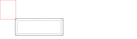
Diagram 1: CCT Shape Barely Touches an Obstacle

In Diagram 1, the red box of the CCT is barely touching the outermost black box of the convex obstacle. In this situation the SQ-Sweep will report an initial overlap but the GQ-Penetration Depth function will report no hit, because the red box is not touching the black box with rounded corners.

To resolve this, inflate the CCT shape for the GQ-Penetration Depth calculation to ensure that it detects an overlap and returns a valid normal. Note that after inflating the CCT shape, the GQ-Penetration Depth function will report that the shapes are penetrated more deeply than they actually are, so take this additional penetration into account when depenetrating in Step 4. This may result in some clipping around the corners and edges of convex objects but the CCT's motion should be acceptable. As the corners/edges become more acute, the amount of clipping will increase.

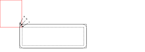
Diagram 2: CCT Overlaps an Obstacle Slightly

Diagram 2 shows a case where the CCT initially overlaps the outer black box seen by the SQ system, but does not overlap the shrunken shape seen by the GQ-Penetration Depth calculator. The GQ-Penetration Depth system will return the penetration from point c to point b but not from point c to point a. Therefore the CCT may clip through the corner of the convex hull after depenetration. This can be corrected in Step 4.

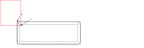
Diagram 3: CCT Overlaps an Obstacle Significantly

As can been seen from Diagram 3, if the CCT penetrates sufficiently that it overlaps with the shrunken shape seen by GQ, the GQ-Penetration Depth calculator will return the penetration from point c to point a. In this case, the GQ-Penetration Depth value can be used without modification in Step 4. However, as this condition would be difficult to categorize without additional computational cost, it is best to inflate the shape as recommended in Step 4 and then subtract this inflation from the returned penetration depth.

Unified MTD Sweep

A recent addition to the scene query sweeps is the flag PxHitFlag::eMTD. This can be used in conjunction with default sweeps to generate the MTD (Minimum Translation Direction) when an initial overlap is detected by a sweep. This flag is guaranteed to generate an appropriate normal under all circumstances, including cases where the sweep may detect an initial overlap but calling a stand-alone MTD function may report no hits. It still may suffer from accuracy issues with penetration depths but, in the cases outlined above around corners/edges, it will report a distance of 0 and the correct contact normal. This can be used to remove components of the sweep moving into the normal direction and then re-sweeping when attempting to implement a CCT. This also generates compound MTDs for meshes/heightfields, which means that it reports an MTD that de-penetrates the shape from the entire mesh rather than just an individual triangle, if such an MTD exists.

Quantizing HeightField Samples

Heightfield samples are encoded using signed 16-bit integers for the y-height that are then converted to a float and multiplied by PxHeightFieldGeometry::heightScale to obtain local space scaled coordinates. Shape transform is then applied on top to obtain world space location. The transformation is performed as follows (in pseudo-code):

localScaledVertex = PxVec3(row * desc.rowScale, PxF32(heightSample) * heightScale,
    col * desc.columnScale)
worldVertex = shapeTransform( localScaledVertex )

The following code snippet shows one possible way to build quantized unscaled local space heightfield coordinates from world space grid heights stored in terrainData.verts:

const PxU32 ts = ...; // user heightfield dimensions (ts = terrain samples)
// create the actor for heightfield
PxRigidStatic* actor = physics.createRigidStatic(PxTransform(PxIdentity));

// iterate over source data points and find minimum and maximum heights
PxReal minHeight = PX_MAX_F32;
PxReal maxHeight = -PX_MAX_F32;
for(PxU32 s=0; s < ts * ts; s++)
{
    minHeight = PxMin(minHeight, terrainData.verts[s].y);
    maxHeight = PxMax(maxHeight, terrainData.verts[s].y);
}

// compute maximum height difference
PxReal deltaHeight = maxHeight - minHeight;

// maximum positive value that can be represented with signed 16 bit integer
PxReal quantization = (PxReal)0x7fff;

// compute heightScale such that the forward transform will generate the closest point
// to the source
// clamp to at least PX_MIN_HEIGHTFIELD_Y_SCALE to respect the PhysX API specs
PxReal heightScale = PxMax(deltaHeight / quantization, PX_MIN_HEIGHTFIELD_Y_SCALE);

PxU32* hfSamples = new PxU32[ts * ts];

PxU32 index = 0;
for(PxU32 col=0; col < ts; col++)
{
    for(PxU32 row=0; row < ts; row++)
    {
        PxI16 height;
        height = PxI16(quantization * ((terrainData.verts[(col*ts) + row].y - minHeight) /
            deltaHeight));

        PxHeightFieldSample& smp = (PxHeightFieldSample&)(hfSamples[(row*ts) + col]);
        smp.height = height;
        smp.materialIndex0 = userValue0;
        smp.materialIndex1 = userValue1;
        if (userFlipEdge)
            smp.setTessFlag();
    }
}

// Build PxHeightFieldDesc from samples
PxHeightFieldDesc terrainDesc;
terrainDesc.format            = PxHeightFieldFormat::eS16_TM;
terrainDesc.nbColumns        = ts;
terrainDesc.nbRows            = ts;
terrainDesc.samples.data    = hfSamples;
terrainDesc.samples.stride    = sizeof(PxU32); // 2x 8-bit material indices + 16-bit height
terrainDesc.thickness        = -10.0f; // user-specified heightfield thickness
terrainDesc.flags            = PxHeightFieldFlags();

PxHeightFieldGeometry hfGeom;
hfGeom.columnScale = terrainWidth / (ts-1); // compute column and row scale from input terrain
                                            // height grid
hfGeom.rowScale    = terrainWidth / (ts-1);
hfGeom.heightScale = deltaHeight!=0.0f ? heightScale : 1.0f;
hfGeom.heightField = physics.createHeightField(terrainDesc);

delete [] hfSamples;

PxTransform localPose;
localPose.p = PxVec3(-(terrainWidth * 0.5f),    // make it so that the center of the heightfield
    minHeight, -(terrainWidth * 0.5f));         // is at world (0,minHeight,0)
localPose.q = PxQuat(PxIdentity);
PxShape* shape = actor->createShape(hfGeom, material, nbMaterials);
shape->setLocalPose(localPose);