Manual¶

Introduction¶

Flex is a particle-based simulation library that is broadly based on Position-Based Dynamics [1], and the Unified Particle Physics for Real-Time Applications SIGGRAPH paper [2].

The core idea of Flex is that everything is a system of particles connected by constraints. The benefit of having a unified representation is that it allows efficient modeling of many different materials, and allows interaction between elements of different types, for example, two-way coupling between rigid bodies and fluids.

Flex’s strength lies in enabling interesting secondary effects that enhance the visual experience. It is not designed to build gameplay affecting physics, for example it lacks functionality such as trigger events, contact callbacks, ray-casting, serialization, etc. Although it is possible to build these capabilities on top of the core solver, they don’t come in the box. For this reason it is recommended to use Flex in conjunction with a traditional rigid-body physics engine, such as PhysX.

The rest of this guide describes the standalone Flex SDK. It discusses some of the common applications, limitations, performance best practices, and general recommendations when using Flex.

Library Design¶

The library is broken into two parts, the core solver (NvFlex.h), which essentially operates on flat arrays of particles and constraints, and an extensions library (NvFlexExt.h), which provides some basic object/asset management to ease integration with typical work flows. The core solver is currently closed source, while the extensions library and demo application are shipped with full source.

The core solver API is written in C-style, and can be considered a low-level wrapper around the solver internals. In contrast to traditional physics APIs, where operations are carried out on one rigid body or constraint at a time, in Flex, all particles and constraints are sent to the solver in one shot, as flat-arrays. This allows Flex to be efficient when dealing with large numbers of constraints and particles, although it means performing incremental updates can be slower.

Flex uses a structure-of-arrays (SOA) data layout for efficiency during simulation. To avoid additional copy overhead the API requires data to be provided in this SOA format.

Quick Start¶

The example code below shows how to initialize the library, create a new solver (similar to a scene in PhysX), and how to tick the solver:

NvFlexLibrary* library = NvFlexInit();

// create new solver
NvFlexSolverDesc solverDesc;
NvFlexSetSolverDescDefaults(&solverDesc);
solverDesc.maxParticles = n;
solverDesc.maxDiffuseParticles = 0;

NvFlexSolver* solver = NvFlexCreateSolver(library, &solverDesc);

NvFlexBuffer* particleBuffer = NvFlexAllocBuffer(library, n, sizeof(float4), eNvFlexBufferHost);
NvFlexBuffer* velocityBuffer = NvFlexAllocBuffer(library, n, sizeof(float4), eNvFlexBufferHost);
NvFlexBuffer* phaseBuffer = NvFlexAllocBuffer(library, n, sizeof(int), eNvFlexBufferHost);

while(!done)
{
        // map buffers for reading / writing
        float4* particles = (float4*)NvFlexMap(particleBuffer, eNvFlexMapWait);
        float3* velocities  = (float3*)NvFlexMap(velocityBuffer, eNvFlexMapWait);
        int* phases = (int*)NvFlexMap(phaseBuffer, eNvFlexMapWait);

        // spawn (user method)
        SpawnParticles(particles, velocities, phases);

        // render (user method)
        RenderParticles(particles, velocities, phases);

        // unmap buffers
        NvFlexUnmap(particleBuffer);
        NvFlexUnmap(velocityBuffer);
        NvFlexUnmap(phaseBuffer);

        // write to device (async)
        NvFlexSetParticles(solver, particleBuffer, NULL);
        NvFlexSetVelocities(solver, velocityBuffer, NULL);
        NvFlexSetPhases(solver, phaseBuffer, NULL);

        // tick
        NvFlexUpdateSolver(solver, dt, 1, false);

        // read back (async)
        NvFlexGetParticles(solver, particleBuffer, NULL);
        NvFlexGetVelocities(solver, velocityBuffer, NULL);
        NvFlexGetPhases(solver, phaseBuffer, NULL);
}

NvFlexFreeBuffer(particleBuffer);
NvFlexFreeBuffer(velocityBuffer);
NvFlexFreeBuffer(phaseBuffer);

NvFlexDestroySolver(solver);
NvFlexShutdown(library);

Although Flex allows you to combine effects in one solver it often makes sense to create a separate one for each type of effect. For example, if you have a scene with clothing and fluids, but they don’t need to interact, you may have one solver for each. This approach provides more flexibility when setting parameters.

Buffers¶

Since Flex 1.1 all data passed to and from Flex must be through a FlexBuffer. This is a simple memory abstraction that allows Flex to support both DirectX, CUDA, and other GPU platforms. To create a buffer use the the NvlexAllocBuffer() method as follows:

NvFlexBuffer* particles = NvFlexAllocBuffer(library, n, sizeof(Vec4), eNvFlexBufferHost);

Buffers must have both their element count and stride set appropriately for the method they are passed to, e.g.: for NvFlexSetParticles(), the method expects a buffer with a stride of sizeof(float)*4.

To send data to Flex you must first map a buffer for reading/writing by calling NvFlexMap(), this will return a pointer to the contents of the buffer which can then be accessed by the CPU code, for example to spawn or update particle data. When the CPU has finished writing to the buffer, it must first unmap the buffer by calling NvFlexUnmap(), and then update the solver by calling a NvFlexSet*() method, e.g.: NvFlexSetParticles(). By calling NvFlexUnmap(), Flex knows the CPU will no longer be accessing the buffer, and it can safely send the new data to the GPU asynchronously.

To retrieve data from Flex you must instruct it to populate a buffer object. For example, to retrieve particle positions you would first call a NvFlexGet*() method, e.g.: NvFlexGetParticles(), and then map it for reading. When you call NvFlexMap() on a buffer with the eNvFlexMapWait flag Flex will block the calling thread until any outstanding transfers have completed. This ensures that you always see the most up to date data.

Why do we use buffers at all? First, they provide an abstraction around graphics APIs that don’t have direct access to raw GPU memory. Second, they allow Flex to ensure transfers are always completed asynchronously and as efficiently as possible.

Particles¶

Particles are the fundamental building-block in Flex. For each particle the basic dynamic quantities of position, velocity, and inverse mass are stored. The inverse mass is stored alongside the position, in the format [x, y, z, 1/m]. In addition to these properties, Flex also stores a per-particle phase value, which controls the particle behavior (see the Phase section for more information). Below is a simple example showing the layout for particle data, and how to set it onto the API.:

NvFlexBuffer* particleBuffer = NvFlexAllocBuffer(library, n, sizeof(Vec4), eNvFlexBufferHost);
NvFlexBuffer* velocityBuffer = NvFlexAllocBuffer(library, n, sizeof(Vec4), eNvFlexBufferHost);
NvFlexBuffer* phaseBuffer = NvFlexAllocBuffer(library, n, sizeof(int), eNvFlexBufferHost);

// map buffers for reading / writing
float4* particles = (float4*)NvFlexMap(particlesBuffer, eNvFlexMapWait);
float3* velocities = (float3*)NvFlexMap(velocityBuffer, eNvFlexMapWait);
int* phases = (int*)NvFlexMap(phaseBuffer, eFlexMapWait);

// spawn particles
for (int i=0; i < n; ++i)
{
        particles[i] = RandomSpawnPosition();
        velocities[i] = RandomSpawnVelocity();
        phases[i] = NvFlexMakePhase(0, eNvFlexPhaseSelfCollide);
}

// unmap buffers
NvFlexUnmap(particleBuffer);
NvFlexUnmap(velocityBuffer);
NvFlexUnmap(phaseBuffer);

// write to device (async)
NvFlexSetParticles(solver, particleBuffer, NULL);
NvFlexSetVelocities(solver, velocityBuffer, NULL);
NvFlexSetPhases(solver, phaseBuffer, NULL);

Radius¶

All particles in Flex share the same radius, and its value has a large impact on simulation behavior and performance. The main particle radius is set via NvFlexParams::radius, which is the “interaction radius”. Particles closer than this distance will be able to affect each other. How exactly they affect each other depends on the other parameters that are set, but this is the master control that sets the upper limit on the particle interaction distance.

Particles can interact as either fluids or solids, the NvFlexParams::solidRestDistance and NvFlexParams::fluidRestDistance parameters control the distance particles attempt to maintain from each other, they must both be less than or equal to the radius parameter.

Phase¶

Each particle in Flex has an associated phase, this is a 32 bit integer that controls the behavior of the particle in the simulation. A phase value consists of a group identifier, and particle flags, as described below:

eNvFlexPhaseGroupMask - The particle group is an arbitrary positive integer, stored in the lower 24 bits of the particle phase. Groups can be used to organize related particles and to control collisions between them. The collision rules for groups are as follows: particles of different groups will always collide with each other, but by default particles within the same group will not collide. This is useful, for example, if you have a rigid body made up of many particles and do not want the internal particles of the body to collide with each other. In this case all particles belonging to the rigid would have the same group value.
eFlexPhaseSelfCollide - To enable particles of the same group to collide with each other this flag should be specified on the particle phase. For example, for a piece of cloth that deforms and needs to collide with itself, each particle in the cloth could have the same group and have this flag specified.
eNvFlexPhaseFluid - When this flag is set the particle will also generate fluid density constraints, cohesion, and surface tension effects with other fluid particles. Note that generally fluids should have both the fluid and self-collide flag set, otherwise they will only interact with particles of other groups.

The API comes with a helper function, NvFlexMakePhase(), that generates phase values given a group and flag set. The example below shows how to set up phases for the most common cases:

// create a fluid phase that self collides and generates density constraints
int fluidPhase = NvFlexMakePhase(0, eNvFlexPhaseSelfCollide | eNvFlexPhaseFluid);

// create a rigid phase that collides against other groups, but does not self-collide
int rigidPhase = NvFlexMakePhase(1, 0);

// create a cloth phase that collides against other groups and itself
int clothPhase = NvFlexMakePhase(2, eNvFlexPhaseSelfCollide);

Active Set¶

Each solver has a fixed maximum number of particles specified at creation time (see NvFlexCreateSolver()), but not all particles need to be active at one time. Before a particle will be simulated, it must be added to the active set. This is an array of unique particle indices that the solver will simulate. Inactive particles have very low computational overhead, so this mechanism can be used to implement more general particle allocation strategies on top of the solver.

The example code below shows how to create an active set which enables simulation on the first 10 particles in the solver:

NvFlexBuffer* activeBuffer = NvFlexAllocBuffer(library, n, sizeof(int), eNvFlexBufferHost);
int* activeIndices = (int*)NvFlexMap(activeBuffer, eNvFlexMapWait);

for (int i=0; i < 10; ++i)
        activeIndices[i] = i;

NvFlexUnmap(activeBuffer);

NvFlexSetActive(solver, activeBuffer, NULL)
NvFlexSetActiveCount(solver, 10);

Note: constraints referencing inactive particles may behave unexpectedly.

Constraints¶

Constraints in Flex are what make particles behave in interesting ways. This section describes the basic constraint types, and discusses how they can be used to model common materials.

Fluids¶

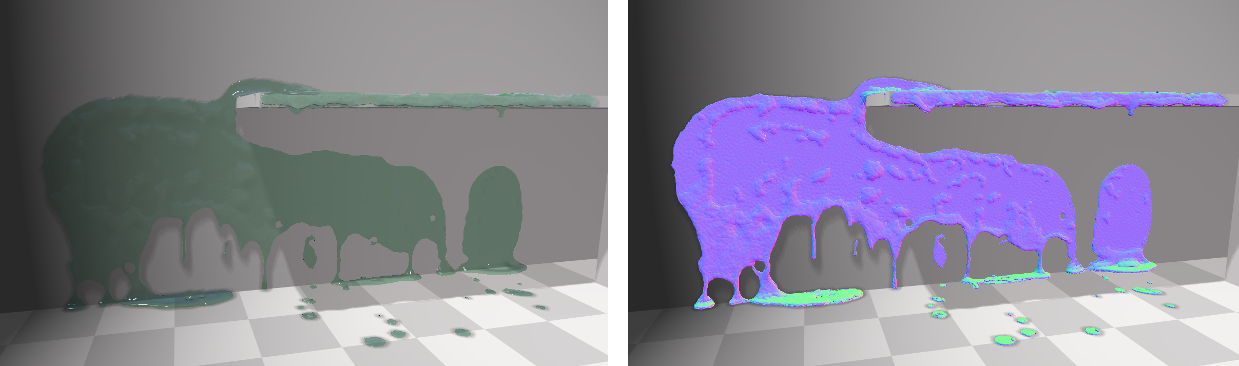
Fluids adhering to a wall

Fluids in Flex are based on Position Based Fluids (PBF) [3]. This method uses position-based density constraints to achieve lower compression and better stability than traditional Smoothed Particle Hydrodynamics (SPH) methods.

The behavior of the fluid depends on the ratio between NvFlexParams::radius and the NvFlexParams::fluidRestDistance, a good rule of thumb is that the ratio should be about 2:1, e.g.: a radius of 10cm, and a rest distance of 5cm. When the radius is large compared to the rest distance the fluid is said to have a larger smoothing distance. Larger smoothing distances generally provide a more accurate simulation, but also tend to be more expensive because particles interact with many more neighbors. If the rest-distance is close to the radius, e.g.: a radius of 10cm, and a rest distance of 9cm, then the fluid will appear more like a granular material than a fluid, but will be cheaper to simulate because there is less overlap between neighbors.

Flex automatically calculates the fluid rest-density from the rest-distance and radius. When seeding fluid particles, the user should just take care to ensure particles are approximately at the rest-distance. In addition to the basic fluid density solve the following fluid behaviors are supported:

Cohesion - Cohesion acts between fluid particles to bring them towards the rest-distance, while the density constraint only acts to push particles apart, cohesion can also pull them together. This creates gooey effects that cause long strands of fluids to form.
Surface Tension - Surface tension acts to minimize the surface area of a fluid. It can generate convincing droplets that split and merge, but is somewhat expensive computationally. Surface tension effects are mostly visible at small scales, so often surface tension is not required unless you have a high-resolution simulation.
Vorticity Confinement - Numerical damping can cause fluids to come to rest unrealistically quickly, especially when using low-resolution simulations. Vorticity confinement works by injecting back some rotational motion to the fluid. It is mostly useful for pools, or larger bodies of water.
Adhesion - Adhesion affects how particles stick to solid surfaces, when enabled particles will stick to, and slide down surfaces. Note that adhesion will affect both fluid and solid particles.

Although Flex does not perform any rendering itself, it can generate information to support high-quality surface rendering based on ellipsoid splatting and screen-space surface reconstruction. If NvFlexParams::smoothing is > 0, then Flex will calculate the Laplacian smoothed fluid particle positions that can be accessed through NvFlexGetSmoothParticles(). If, NvFlexParams::anisotropyScale is > 0, then Flex will also calculate the anisotropy vectors for each fluid particle according to the distribution of it’s neighbors, these can be accessed through NvFlexGetAnisotropy(). See [4] for more information on the anisotropy calculation, and refer to the demo application for example OpenGL fluid rendering code.

Springs¶

Springs in Flex are specified as pairs of particle indices, a rest-length, and a stiffness coefficient. They are not a spring in the classical sense, but rather a distance constraint with a user-specified stiffness. The index pairs should appear consecutively, for example the following example code sets up a chain of particles with each edge 1 unit long, with a stiffness coefficient of 0.5:

const int springIndices[] = { 0, 1, 1, 2, 2, 3 }
const float springLengths[] = { 1.0f, 1.0f, 1.0f }
const float springCoefficients[] { 0.5f, 0.5f, 0.5f }

NvFlexBuffer indicesBuffer = NvFlexAllocBuffer(library, 6, sizeof(int), eNvFlexBufferHost);
NvFlexBuffer lengthsBuffer = NvFlexAllocBuffer(library, 3, sizeof(float), eNvFlexBufferHost);
NvFlexBuffer coefficientsBuffer = NvFlexAllocBuffer(library, 3, sizeof(float), eNvFlexBufferHost);

memcpy(NvFlexMap(indicesBuffer, eNvFlexMapWait), springIndices, sizeof(springIndices));
memcpy(NvFlexMap(lengthsBuffer, eNvFlexMapWait), springLengths, sizeof(springLengths));
memcpy(NvFlexMap(coefficientsBuffer, eNvFlexMapWait), springCoefficients, sizeof(springCoefficients));

NvFlexUnmap(indicesBuffer);
NvFlexUnmap(lengthsBuffer);
NvFlexUnmap(coefficientsBuffer);

NvFlexSetSprings(solver, indicesBuffer, lengthsBuffer, coefficientsBuffer, 3);

Distance constraints are incredibly versatile, and relatively cheap to solve. When combined with dynamic topology changes they can model interesting effects such as tearing, merging.

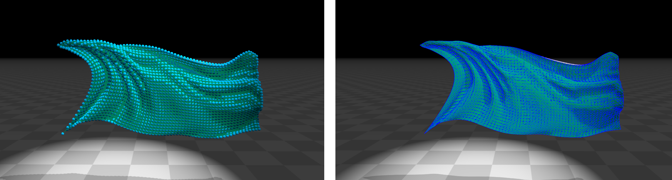
Cloth¶

Clothing in Flex is modeled using networks of springs. The cloth model is up to the user, but the extensions library provides an example cloth cooker (NvFlexExtCreateClothFromMesh()) that implements a common approach where the 1-ring neighbors are used to control stretch, and 2-ring neighbors are used to control bending.

Cloth Flag

In addition to the basic cloth behavior governed by the distance constraints, there are some cloth specific features in Flex. By specifying the underlying triangle topology using NvFlexSetDynamicTriangles(), additional forces can be computed to generate more complex effects. Specifically:

Lift and drag - Triangles will generate drag forces and lift forces proportional to area and orientation. This can generate interesting fluttering motion on pieces of cloth, typically drag forces should be set higher than lift.
Wind - In addition to gravity, a global acceleration vector is provided to model basic wind. If the drag parameter is non-zero then triangles will receive forces according to the wind vector’s direction and magnitude.
Smooth normals - When triangle topology is set, Flex will also generate smoothed vertex normals based on the current particle positions, these can be retrieved through NvFlexGetNormals() for rendering.

Note: because all collisions in Flex are performed at the particle level, the cloth mesh must be sufficiently well tessellated to avoid particle tunneling. Care must especially be taken for clothing with self-collision, the cloth mesh should be authored so that the mesh has a uniform edge length close to the solid particle rest distance. If self-collision is enabled, and particles are closer than this in the mesh then erroneous buckling or folding might occur as the distance and collision constraints fight each other.

Inflatables¶

Inflatable bodies can be seen as an extension of a cloth model. An inflatable can be constructed by starting with a closed triangle mesh and adding a volume constraint to the solver. To set up an inflatable object Flex needs a closed, 2-manifold mesh to be specified using NvFlexSetDynamicTriangles(). An inflatable is then defined by a start and end range in the triangles array using NvFlexSetInflatables(). Each inflatable has an ‘overpressure’ parameter that controls how inflated it is relative to it’s rest volume.

Although Flex does not currently expose tetrahedral constraints, they can be simulated in a limited fashion by creating distance constraints along the tetrahedral mesh edges.

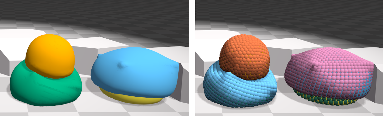
Rigid Bodies¶

Rigid bodies in Flex are modeled quite differently from traditional rigid body solvers. In Flex, each rigid body consists of a collection of particles, and a shape matching constraint that holds them in a rigid configuration. By using particles to represent rigid bodies, Flex can use the same collision pipeline as for fluids, clothing, etc. Also, the shape-matching allows us to have semi-rigid, or deformable bodies, by setting a stiffness parameter per-body.

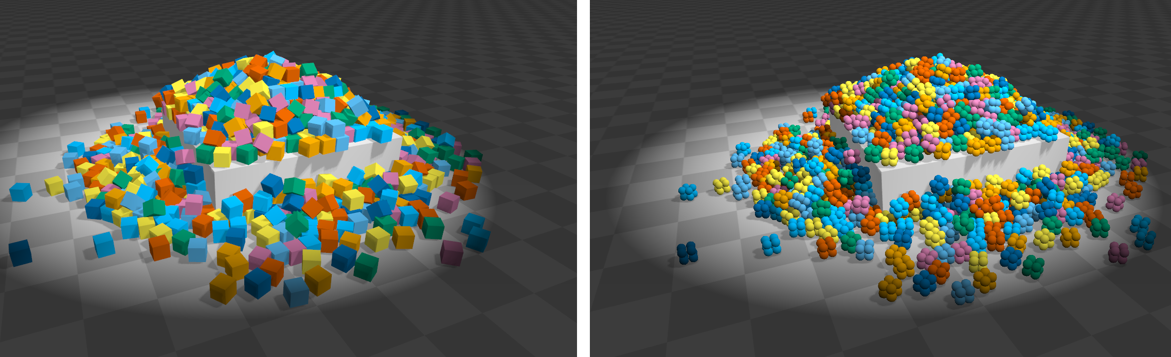
Block Pile

Rigid bodies are specified by a set of rest-positions, relative to the body center of mass, through NvFlexSetRigids(). The extensions library provides an example function (NvFlexExtCreateRigidFromMesh()) that shows how particles can be placed to represent a triangle mesh. During simulation collisions are handled for each particle individually, so that after a collision, the particles are typically no-longer in their rigid configuration. In order to restore rigidity, the least squares best rigid transform is found to match the deformed particle positions back to the rigid shape. Unlike a traditional rigid body solver the linear or angular velocity of the body are not explicitly tracked, these quantities are simply derived from the particles referenced.

There are some limitations with this particle based approach. When the time-step is too large the particles can tunnel through each other and become interlocked. Flex allows you to specify a normal and distance value per-particle to help avoid this, see the paper [2] for more details. Another limitation of shape-matching is that the stiffness of the rigid body is affected by how many particles make it up. Bodies made of many particles can require many iterations to converge, and appear ‘squishy’. Because of this, it is generally recommended to use Flex for smaller rigid bodies, and use a traditional rigid body solver for larger bodies. A good rule of thumb is to keep the effective particle resolution under 64^3 per-body.

The table below summarizes the strengths and weaknesses of Flex rigid bodies and suggests some suitable applications:

Strength	Examples
Environmental debris	Bullet shrapnel, rocks, cans
Unstructured piling	Piles of trash
Non-convex shapes	Irregular stones, bones, bananas
Two-way interaction	Parachuting bunnies

Weakness	Examples
Thin or sharp objects	Floor tiles, glass shards
Structured stacking	Brickwork, arches
Large relative sizes	Large scale destruction
Collision filtering	Character controller

The particles in a rigid body can be affected by other constraints in Flex, some example applications of this generality are:

Adding a rigid constraint to a piece of clothing to generate stiff bending resistance even at low-iteration counts
Adding a rigid constraint to a fluid and animating the rigid stiffness to simulate melting or phase changes
Connecting rigid bodies to clothing through distance constraints, e.g.: cloth hanging from the sides of a rigid body

Soft Bodies¶

Soft bodies can be modelled by using ‘clusters’ of shape-matching constraints. Because each shape-matching constraint’s output is a rotation and translation, it can be useful to think of them similar to bones in a traditional skeletal deformation system.

Each paticle may belong to multiple clusters (shape-matching constraint), by overlapping clusters and averaging their output the system can deform realistically. The more shape-matching constraints used in body the more degrees of freedom it has. If a body has only one shape-matching constraint then it is treated essentially as a rigid body.

The Flex extensions library contains an example cooker for creating soft bodies, see NvFlexExtCreateSoftFromMesh(). It works by first voxelizing the mesh into particles, then grouping particles into overlapping clusters. Because shape matching consraints act to resist bending and torsion in the model the cooker may optionally include regular distance constraints, or ‘links’ between neighboring particles. By setting the stiffness separately for links and clusters bending and stretching can be controlled separately.

Solver¶

Time Stepping¶

Flex supports sub-stepping through the NvFlexUpdateSolver() substeps parameter. There is a trade-off between increasing the number of iterations and increasing the number of substeps. Collision detection is performed once per-substep, which means increasing substeps is more expensive than adding iterations, but it is often the only way to improve the accuracy of collision detection when using small particles. Each substep performs NvFlexParams::numIterations solve passes over the constraints, so substepping will also make constraints appear stiffer.

For best results the solver should be ticked with fixed time-steps. If the application runs with a variable frame rate, then the application should divide each frame’s delta time into fixed size chunks and set the sub-step parameter accordingly. Variable time stepping is supported, but will often result in ‘wiggle’ or ‘jittering’, as the amount of constraint error is usually related to the time-step size.

Note: many constraint types allow the user to specify a stiffness value, but the overall stiffness of the simulation is dependent on the number of solver iterations, the time-step, and the number of sub-steps.

Relaxation¶

Typically the constraint solve is the most time-consuming aspect of the simulation, so Flex has some parameters to fine-tune the convergence speed. The solver has two primary modes of operation, local, and global, as described below:

eNvFlexRelaxationLocal - In this mode a local averaging is performed per-particle. The sum of all constraints affecting a particle is averaged before updating the position and velocity. This method is very robust and will generally converge even in difficult circumstances, for example when competing or redundant constraints are present. However it tends to converge quite slowly, and requires many iterations to appear stiff. To improve convergence in this mode NvFlexParams::relaxationFactor can be set to a value > 1.0, this is called over relaxation, values much larger than 1.0 will occasionally cause the simulation to blow up so it should be set carefully.
eNvFlexRelaxationGlobal - In this mode the effect of constraints is weighted by a global factor, no averaging is performed. This mode tends to converge faster than the local mode, but may cause divergence in difficult cases. In this mode the relaxation factor, relaxationFactor, should be set to a value < 1.0, e.g.: 0.25-0.5 to ensure convergence.

Collision¶

Flex supports static collision geometry in the form of spheres, capsules, planes, convex shapes, triangle meshes, and signed distance fields (SDF). Shape geometry is always specified in a local space, and then instanced into the scene with a translation and rotation. Flex uses a flat buffer of geometry types to allow it to efficiently treat each type:

union NvFlexCollisionGeometry
{
        NvFlexSphereGeometry sphere;
        NvFlexCapsuleGeometry capsule;
        NvFlexBoxGeometry box;
        NvFlexConvexMeshGeometry convexMesh;
        NvFlexTriangleMeshGeometry triMesh;
        NvFlexSDFGeometry sdf;
};

The collision geometry is specified as an array of geometry and world space transforms. Once an array of geometry structs and transforms has been filled out it is sent to Flex via the NvFlexSetShapes() method. This will build a broad-phase structure that allow for fast GPU queries against the shapes. The following example shows how to set up a sphere and a triangle mesh shape:

NvFlexCollisionGeometry* geometry = (NvFlexCollisionGeometry*)NvFlexMap(geometryBuffer, 0);
float4* positions = (float4*)NvFlexMap(positionsBuffer, 0);
quat* rotations = (quat*)NvFlexMap(rotationsBuffer, 0);
int* flags = (int*)NvFlexMap(flagsBuffer, 0);

// add sphere
flags[0] = NvFlexMakeShapeFlags(eNvFlexShapeSphere, false);
geometry[0].sphere.radius = radius;
positions[0] = float3(0.0f);
rotations[0] = quat(0.0f);

// create a triangle mesh
NvFlexTriangleMeshId mesh = NvFlexCreateTriangleMesh();
NvFlexUpdateTriangleMesh(lib, mesh, vertices, indices, numVertices, numTriangles, NULL, NULL);

// add triangle mesh instance
flags[1] = NvFlexMakeShapeFlags(eNvFlexShapeTriangleMesh, false);
geometry[1].triMesh.mesh = mesh;
geometry[1].triMesh.scale[0] = 1.0f;
geometry[1].triMesh.scale[1] = 1.0f;
geometry[1].triMesh.scale[2] = 1.0f;
positions[1] = float3(0.0f, 100.0f, 0.0f);
rotations[1] = quat(0.0f);

// unmap buffers
NvFlexUnmap(geometryBuffer, 0);
NvFlexUnmap(positionsBuffer, 0);
NvFlexUnmap(rotationsBuffer, 0);
NvFlexUnmap(flagsBuffer, 0);

// send shapes to Flex
NvFlexSetShapes(solver, geometry, positions, rotation, NULL, NULL, flags, 2);

Shapes may also have a previous translation and rotation specified which enables accurate frictional effects to be calculated. Each shape may also be marked as static or dynamic, which affects the priority that contacts are solved in, see the section on collision priorty;

Spheres¶

The simplest shape, defined as follows:

struct NvFlexSphereGeometry
{
        float radius;
};

Capsules¶

Defined as a radius and half-height along the local x-axis, with the center of the shape at middle of the capsule:

struct NvFlexCapsuleGeometry
{
        float radius;
        float halfHeight;
};

Triangle Meshes¶

Indexed triangle meshes can be created by calling the NvFlexCreateTriangleMesh() method. Once a mesh definition has been created it can be instanced into the scene using the following structure:

struct NvFlexTriangleMeshGeometry
{
        float scale[3];            //!< The scale of the object from local space to world space
        FlexTriangleMeshId mesh;   //!< A triangle mesh pointer created by NvFlexCreateTriangleMesh()
};

Collision against triangle meshes is performed using CCD line-segment tests, using the particle velocity at the beginning of the frame. Triangle tests are performed as if one-sided with CCW front faces. Even though the initial test is a form of continuous collision detection, it is still possible for particles to tunnel if they are pushed through the triangle mesh by constraints during the constraint solve.

Note: For triangle mesh collision to be robust, the NvFlexParams::collisionDistance should be set to a non-zero value, otherwise particles may initially collide and then ‘slip’ through the mesh due to numerical precision errors.

Convex Meshes¶

Convex polyhedrons are supported, and are represented by sets of half-spaces specified by the following plane struct:

struct NvFlexConvexMeshGeometry
{
        float scale[3];
        NvFlexConvexMeshId mesh;
};

Where the mesh is created through NvFlexCreateConvexMesh().

Signed Distance Fields¶

Signed distance fields (SDFs) can be specified as a dense voxel array of floating point data. SDFs are very cheap to collide against because they are stored as volume textures on the GPU and have an O(1) lookup cost. To create an SDF, first call NvFlexCreateSDF(), and then instance it into the scene by filling out the geometry struct:

struct NvFlexSDFGeometry
{
        float scale;                                    //!< Should be equivalent to the width of the SDF in world space.
        NvFlexDistanceFieldId field;    //!< A signed distance field pointer created by NvFlexCreateSDF()
};

SDFs are defined in a right-handed coordinate system where the voxel corresponding to an index x,y,z is given by index = z*width*height + y*width + x. The origin of the shape is at the corner of the SDF with index 0,0,0.

Currently SDFs can only be square (cubic) volumes, the scale parameter should be set equal to the edge length of the shape AABB.

Flex uses the convention that negative values represent the shape interior, with the distance value normalized between -1 to 1 according to the volume dimensions.

Planes¶

In addition to the convex meshes, there is also a convenient way to set infinite half-spaces to the solver through NvFlexParams::planes.

Margins¶

For most geometry, Flex uses discrete collision detection which is generally performed once per-substep. Performing collision detection only once per-substep is efficient, but means that collisions may be missed. When this happens, the particle may either tunnel through the shape, or be ejected back out on the next frame. This can sometimes appear as popping or jumping for no obvious reason. One way to ensure collisions are not missed is to increase the distance at which the contacts are generated. This is what the margin parameters are used for:

NvFlexParams::particleCollisionMargin - Increases the distance at which particle interactions are created
NvFlexParams::shapeCollisionMargin - Increases the distance at which contacts with static geometry are considered

Note: increasing the collision margin will naturally generate more contacts, which can also be problematic. Internally Flex stores up to 6 contact planes per-particle, if this is exceeded then subsequent contacts will be dropped. Increasing the margin can also harm performance, be particularly careful increasing the particle collision margin, as this can cause many particle neighbors to be unnecessarily considered. Generally the margins should only be increased if you are having problems with collision, and always set as low as possible.

Note: margins are added on top of the NvFlexParams::radius parameter.

Priority¶

The order in which particle contacts with shapes are processed has a large impact on the behavior of the simulation. To avoid tunneling through thin shapes, and to prevent dynamic objects pushing particles through static shapes, Flex processes contacts with the following priority:

Triangle meshes
Static signed distance fields (SDFs)
Static convex meshes
Dynamic convex meshes

Diffuse Particles¶

Diffuse foam and spray particles

The spray and foam in Flex is made through the use of diffuse particles. These are secondary, passive, particles that can be used to add additional detail to an underlying simulation. Diffuse particles can be created through the NvFlexSetDiffuseParticles() method, or created by the simulation itself. If NvFlexParams::diffuseThreshold is set, then colliding fluid particles generate a diffuse potential according to their kinetic energy and relative velocity. When this potential goes over the threshold a new diffuse particle will be spawned at a random location around that particle.

When a diffuse particle is surrounded by fluid neighbors, it will interpolate their velocity and be advected forward through the flow. If a diffuse particle has less than NvFlexParams::diffuseBallistic neighboring particles, then it will be treated as a simple ballistic particle and move under gravity.

Note: it is often useful to have the diffuse particles sorted back to front for rendering. The solver can optionally perform this sort by specifying the NvFlexParams::diffuseSortAxis, if this is zero then the particles will not be sorted for rendering.

Threading¶

The Flex core and extension APIs are not thread-safe, meaning only one thread should ever use the API at a time. Almost all Flex operations are performed asynchronously on the GPU. For example, when you call NvFlexUpdateSolver() Flex will launch a number of GPU kernels that will complete some time in the future. Likewise, when you ask Flex to get the updated data using one of the NvFlexGet*() methods, it is launching an asynchronous copy into the FlexBuffer provided. Control will return to the CPU while the transfer is still in progress.

Synchronization occurs when you call NvFlexMap() on a simulation buffer. To avoid making the CPU wait a long time for the GPU to finish its work it is good practice to call NvFlexMap() as far away from the NvFlexUpdateSolver() and NvFlexGet*() as possible. This gives the GPU enough time to finish its work so that the new data is ready for when you call NvFlexMap(). The following snippet shows an example of this by performing the main game tick after the the read-back methods have been issued.:

while (!done)
{
// map buffers for reading / writing (synchronizes with GPU)
float4* particles = (float4*)NvFlexMap(particleBuffer, eNvFlexMapWait);
float3* velocities  = (float3*)NvFlexMap(velocityBuffer, eNvFlexMapWait);
int* phases = (int*)NvFlexMap(phaseBuffer, eNvFlexMapWait);

// application CPU-side particle update
UpdateBuffers(particles, velocities, phases);

// unmap buffers
NvFlexUnmap(particleBuffer);
NvFlexUnmap(velocityBuffer);
NvFlexUnmap(phaseBuffer);

// write to device (async)
NvFlexSetParticles(solver, particleBuffer, NULL);
NvFlexSetVelocities(solver, velocityBuffer, NULL);
NvFlexSetPhases(solver, phaseBuffer, NULL);

// tick (async)
NvFlexUpdateSolver(solver, dt, 1, NULL);

// read back (async)
NvFlexGetParticles(solver, particleBuffer, NULL);
NvFlexGetVelocities(solver, velocityBuffer, NULL);
NvFlexGetPhases(solver, phaseBuffer, NULL);

// Perform CPU work here while update and transfer are in flight
TickGame()
}

Note: Flex can also transfer data directly to OpenGL or DirectX buffers directly through the CUDA-graphics interop mechanism, see the CUDA programming guide and Flex demo application for more details.

Profiling¶

Because Flex executes most of its work asynchronously on the GPU, it is not recommended to measure execution times with CPU timers around API calls. GPU kernel timers can be retrieved by first passing true to the timers parameter of NvFlexUpdateSolver(), and then calling NvFlexGetTimers(). The returned NvFlexTimers structure has timers for each stage of the simulation, these timers can give a good idea of which parts of the update pipeline are the bottleneck.

Note: Enabling timers can have a negative impact on overall performance (although individual timers will be accurate), it is recommended to use timers only when profiling.

Limitations / Known Issues¶

Position-Based Dynamics has a close relationship to traditional implicit time-stepping schemes. As such, it is quite dissipative and will quickly lose energy, often this is acceptable (and sometimes desirable), however external forcing functions (such as vorticity confinement) can be used to inject energy back to the simulation.
Flex is not deterministic. Although simulations with the same initial conditions are often reasonably consistent, they may diverge over time, and may differ between different GPU architectures and versions.
Restitution for rigid bodies may behave weaker than expected, this is generally problematic for shape-matched rigid bodies.
Particles can have a maximum of 6 contact planes per-step, if a particle overlaps more than 6 planes then contacts will be dropped.

Acknowledgments¶

The Flex demo application uses the imgui library from Mikko Mononen’s Recast library, https://github.com/memononen/recastnavigation
The Flex demo application uses the stb_truetype.h font library from Sean Barrett, https://github.com/nothings/stb
The Flex demo application uses the SDL library, https://www.libsdl.org
The Flex solver uses NVIDIA’s CUB library for parallel operations internally, http://nvlabs.github.io/cub/

References¶

[1] Position Based Dynamics - Matthias Müller, Bruno Heidelberger, Marcus Hennix, John Ratcliff - J. Vis. Communications, 2007 - http://dl.acm.org/citation.cfm?id=1234575

[2] Unified Particle Physics for Real-Time Applications - Miles Macklin, Matthias Müller, Nuttapong Chentanez, Tae-Yong Kim: Unified Particle Physics for Real-Time Applications, ACM Transactions on Graphics (SIGGRAPH 2014), 33(4), http://dl.acm.org/citation.cfm?id=2601152

[3] Position Based Fluids - Miles Macklin, Matthias Müller: Position Based Fluids, ACM Transactions on Graphics (SIGGRAPH 2013), 32(4), http://dl.acm.org/citation.cfm?id=2461984

[4] Reconstructing surfaces of particle-based fluids using anisotropic kernels - Jihun Yu and Greg Turk. 2013. ACM Trans. Graph. 32, 1, Article 5 (February 2013). http://dl.acm.org/citation.cfm?id=2421641

Table Of Contents

Previous topic

Next topic

Manual¶

Introduction¶

Library Design¶

Quick Start¶

Buffers¶

Particles¶

Radius¶

Phase¶

Active Set¶

Constraints¶

Fluids¶

Springs¶

Cloth¶

Inflatables¶

Rigid Bodies¶

Soft Bodies¶

Solver¶

Time Stepping¶

Relaxation¶

Collision¶

Spheres¶

Capsules¶

Triangle Meshes¶

Convex Meshes¶

Signed Distance Fields¶

Planes¶

Margins¶

Priority¶

Diffuse Particles¶

Threading¶

Profiling¶

Limitations / Known Issues¶

Acknowledgments¶

References¶

Table Of Contents

Previous topic

Next topic

Quick search

Manual¶

Introduction¶

Library Design¶

Quick Start¶

Buffers¶

Particles¶

Radius¶

Phase¶

Active Set¶

Constraints¶

Fluids¶

Springs¶

Cloth¶

Inflatables¶

Rigid Bodies¶

Soft Bodies¶

Solver¶

Time Stepping¶

Relaxation¶

Collision¶

Spheres¶

Capsules¶

Triangle Meshes¶

Convex Meshes¶

Signed Distance Fields¶

Planes¶

Margins¶

Priority¶

Diffuse Particles¶

Threading¶

Profiling¶

Limitations / Known Issues¶

Acknowledgments¶

References¶